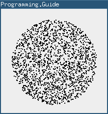
Generating a random point within a circle (uniformly)

For a circle of radius R you do:

double a = random() * 2 * PI
double r = R * sqrt(random())

// If you need it in Cartesian coordinates
double x = r * cos(a)
double y = r * sin(a)

where random() gives a uniformly random number between 0 and 1.

Why sqrt(random())?

Let's look at the math that leads up to sqrt(random()). Assume for simplicity that we're working with the unit circle, i.e. R = 1.

The average distance between points should be the same regardless of how far from the center we look. This means for example, that looking on the perimeter of a circle with circumference 2 we should find twice as many points as the number of points on the perimeter of a circle with circumference 1.

Since the circumference of a circle (2πr) grows linearly with r, it follows that the number of random points should grow linearly with r. In other words, the desired probability density function (PDF) grows linearly. Since a PDF should have an area equal to 1 and the maximum radius is 1, we have

So we know how the desired density of our random values should look like. Now: How do we generate such random values when all we have is a function that produces values between 0 and 1?

We use a trick called inverse transform sampling. An intuitive explanation of how this method works can be found here: Generating a random value with a custom distribution.

Step 1: Create the cumulative distribution function (CDF)

The CDF is, as the name suggests, the cumulative version of the PDF. Since we're working with reals, the CDF is expressed as an integral.

CDF(x) = ∫PDF = ∫2x = x²

Step 2: Mirror the CDF along y = x

Mathematically this boils down to swapping x and y and solving for y:

CDF:y = x²
Swap:x = y²
Solve:y = √x
CDF^-1:y = √x

Step 3: Apply the resulting function to a uniform value between 0 and 1

CDF^-1(random()) = √random()

And that's where sqrt(random()) comes from.